Short Samples:
The Politics of Climate Change (Anthony Giddens)
(February 20th, 2014. The version of T-LAB used was 9.1)
This
short example consists of a sort of exercise through which, while analysing
a popular book of the sociologist Anthony Giddens (i.e. The
Politics of Climate Change), we focus on methodological issues concerning
the use of some T-LAB
tools for text analysis.
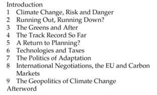
The book in question consists of an introduction, nine chapters and an afterword
(see Fig. 1 below).
That means that - at the source - there are eleven ordered sections that the
whole discourse of the author is subdivided into.
Consequently, in T-LAB jargon, the book is a corpus
which - via a categorical variable - is partitioned
into eleven subsets.
Fig.
1
As
a starting point (see section 1 below), we will
explore some similarities and differences between these
eleven subsets and we will map their relationships accordingly.
Subsequently
(see section 2 below), by assuming that the various
subsets (i.e. book chapters) exhibit the mains ‘themes’ (or ‘topics’)
in different proportion, we will consider as analysis units text segments which
roughly correspond to a couple of sentences (Click
here for more information) and we will partition the book
contents into thematic clusters consisting of such analysis units.
Finally
(see section 3 below), by using some new
features of T-LAB 9.1, the dynamic
sequence of themes both within the entire book and their chapters will
be explored.
SECTION 1: DEALING WITH BOOK CHAPTERS
A key point to keep in our mind is that – at every step of our exercise
- each analysis unit (i.e. a book chapter, a text
segment, a theme, etc.) can be represented as a feature
vector, that is as a vector of term weights. And this is the very reason
why lots of techniques for automated text analysis can apply algorithms for
pattern recognition.
Actually,
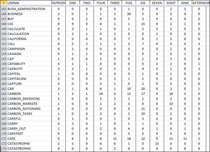
after the preprocessing phase, a contingency table is easily obtained (see Fig.
2 below), the rows of which correspond to key-words (i.e. terms) and the columns
of which correspond to the sections that the Giddens book is subdivided into
(i.e. eleven). So, in this case, each column is a vector the features of which
(i.e. words) have a weight which corresponds to their occurrences within a chapter
of the book. (N.B.: Depending on the type of analysis, various kinds of normalized
weights can be obtained by using the T-LAB
tools. For example, a clustering tool uses the TF-IDF
and the Euclidean norm, the Correspondence Analysis
tool uses the Chi-square distance, etc.).
More
specifically, in our case, we use a list which includes
1,457 key words obtained through an automatic lemmatization
process (e.g. the lemma ‘change’ includes all occurrences of distinct
words like ‘change’, ‘changes’, ‘changing’, ‘changed’).
As a ‘golden standard’, such a list doesn’t include stop-words
(e.g. articles, prepositions etc.), but it does include word phrases and multi-word
expressions like ‘global_warming’, ‘European_Commission’,
‘level_of_emissions’ and so on.
In our case, the lower occurrence value of the listed key-words is 5.
Fig.
2 (Click
here to download the above contingency table as .csv table)
In
order to get a initial picture of the book contents,
a simple Correspondence Analysis
is performed which allows us to map the relationships between all rows and all
columns of the above table, as well as to explore the hidden variables (i.e.
the factors) which frame the Giddens discourse and - at the same time - refer
to a sort of socio-cultural dialectics.
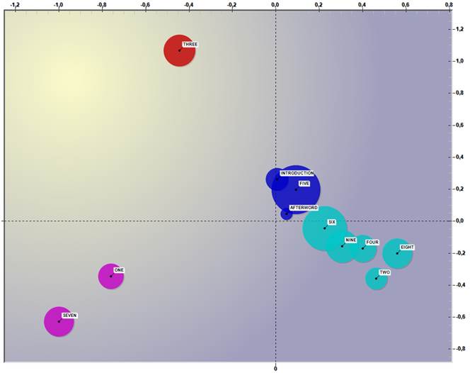
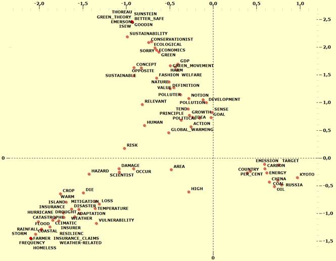
For
example, the following two maps illustrate how both the relationships between
corpus subsets and the relationships between key-words are rearranged through
the semantic oppositions of the first two factors.
Fig.
3
Fig.
4
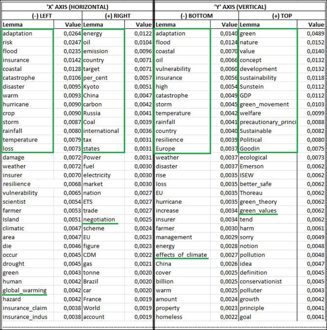
The
semantic characteristics of the first two factors, respectively ‘X’
(abscissa, horizontal) and ‘Y’ (ordinate, vertical), and their oppositions
are summarized by tables listing the absolute contributions
of the characteristic words onto the factorial poles (see below).
Fig.
5
In
short, we may say that the first bipolarity (i.e. the ‘X’ axis) concerns
the ‘risks’ of the climate change on
the left side and its ‘policy’ on the
right side, whereas the second bipolarity (i.e. the ‘Y’ axis) concerns
the experienced ‘effects’ on the bottom
side and the values of ‘sustainable development’
on the top side.
Actually,
because the shape produced by the first two factors resembles to a 'Y' sloping
on the left side, there is a slight difference between 'risks' and 'effects'.
So, as
the ‘specific’ positions of some chapters on the map in Fig. 3 above
are quite intriguing (see chapter three in the top-left quadrant, chapters one
and seven in the bottom-right), we are interested in checking their characteristics.
More specifically, by using the Specificity
Analysis tool which applies the chi-square test to the intersections of
the contingency table depicted in Fig. 2, we are enabled to list the ‘typical
words’ of the above mentioned chapters.
Ordered
by decreasing chi-square values, the top ten typical words
of the three chapters in question (i.e. the words which, through a comparison
with the entire corpus, result to be significantly ‘over used’ within
these subsets) result to be the following:
green
nature
concept
value
sustainability
GDP
development
Sustainable
precautionary_principle
green_movement
adaptation
flood
insurance
coastal
hurricane
catastrophe
crop
loss
insurer
disaster
(*) ‘IPCC’
is the acronym of ‘Intergovernmental Panel on Climate
Change’.
By computing
normalized TF-IDF values, the above mentioned T-LAB
tool allows us also to extract the most significant text segments of three chapters
in question. In this case, just as an example, we report the first of each (i.e.
those with the highest TF-IDF score).
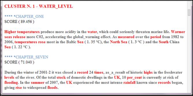
CHAPTER
ONE
Higher temperaturesproduce more acidity in thewater, which couldseriouslythreatenmarinelife.Warmerseasrelease moreC02, accelerating the global_warmingeffect. As measured over the period from 1982 to 2006,temperaturesrose most in the BalticSea(1. 35 °C), the NorthSea(1. 3 °C) and the South ChinaSea(1. 22 °C).
CHAPTER
THREE
In bothsenses, 'development' meansthe accumulation ofwealth, normallymeasuredin_terms_ofGDP, such_that asociety becomes progressively richer. Itimpliesthat thiswealthis generated in some large part by theeconomictransformation of thesociety inquestion, as a self-perpetuating
process.
CHAPTER
SEVEN
During the winter of 2001-2 it wasclosedarecord24 times, as_a_result
of historichighsin the freshwaterlevelsof the river. Of thetotalstock of domestic dwellings in theUK, 10 per_cent is currently atriskofflooding. In the summer of 2007, theUKexperienced the most intenserainfallknown sincerecordsbegan, givingriseto widespreadfloods.
Before
going further, it is worth recalling that some T-LAB
tools allow us to explore the word co-occurrence relationships
within each corpus subset.
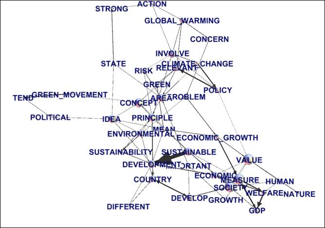
For
example, by selecting a short list of key words (i.e. those with an occurrence
value => 10), the internal relationships within chapter three, can be plotted
either by means of a MDS
method (see Fig. 6 below) or by means of Network Analysis
(see Fig. 7 below).
Fig.
6
Fig.
7
N.B.:
The above graph has been realized through Gephi
(http://gephi.org/) by importing a .gml
file created by T-LAB.
SECTION
2: DEALING WITH THEMES
Let’s now
try to perform a thematic analysis of the Giddens
book.
Actually T-LAB
includes a specific tool (i.e. Thematic
Analysis of Elementary Contexts) which allows us to do this in a easy and
straightforward way; however, by considering the didactic nature of this example,
we have decided to proceed otherwise and provide the reader with all technical
details.
As is known, when
talking of ‘automated’ thematic analysis, if our aim is to assign
each analysis unit to a fixed category (i.e. a theme), three key points must
be clarified in advance:
a) which
analysis units to consider;
b) which
categories to use;
c) which
algorithms to apply.
In relation to
the above point (a) we use the text segments automatically provided by T-LAB
(see, for example, the three characteristic elementary
contexts quoted at the end of the previous section 1).
With regards to
points ‘b’ and ‘c’, as both call into question the difference
between supervised and unsupervised
methods (i.e. between methods which use pre-defined categories and methods which
seek patterns in the data), we use a hybrid approach
consisting of the following steps:
1- two
unsupervised methods are applied which allow us to extract the main themes
of the book and to describe each of these themes by means of feature vectors.
The two methods, both implemented in T-LAB, are:
the bi-secting K-means clustering and the topic
model.
More specifically,
two different T-LAB tools ( i.e. the Thematic
Analysis of Elementary Contexts , which uses the bi-secting K-means algorithm,
and Modeling of Emerging Themes ,which
uses the Latent Dirichlet Allocation and the Gibbs Sampling for the topic analysis)
allow the user to export dictionaries the feature
vectors of which consist of term weights obtained by using either the Chi-square
values (unsupervised clustering) or the probability values (topic model).
2- two
supervised classifications of text segments are performed: the first
one by using the feature vectors describing the clusters,
the second one by using the feature vectors describing the topics.
More details will be provided below.
3- the results
of the above two classifications are compared and
one of them is used for further analyses.
In order to compare
the results provided by the two unsupervised methods (see ‘1’
above), we decide to obtain the same number (i.e. twelve) of ‘themes’/’topics’,
and so the same number of feature vectors describing each of them.
As explained in
the T-LAB Manual/Help,
in the case of supervised classification (see ‘2’ above), the analysis
steps are the following:
a) normalization
of the seed vectors corresponding to the 'k' categories of the dictionary used;
b) computation
of Cosine similarity and of Euclidean distance between each 'i' context unit
(i.e. text segment) and each 'k' seed vector;
c) assignment
of each 'i' context unit to the 'k' class or category for which the corresponding
seed is the closest (In this case, maximum Cosine similarity and minimum Euclidean
distance must coincide, otherwise T-LAB consider
the 'i' context unit as unclassified).
In our case the
above three steps are repeated twice: the first time by applying the category
dictionary obtained by the unsupervised clustering, the second time by
applying the category dictionary obtained by the topic model.
Some measures
provided by T-LAB (i.e. Calinski-Harabasz, Davies-Bouldin,
McClain-Rao and Silhouette indexes) allow us to compare
the two partitions obtained by the above mentioned unsupervised methods
and – as a result - their quality doesn’t
appear to be significantly different.
However, after having evaluated the semantic coherence
of the two solutions, we decide to use the partition obtained by using the dictionary
extracted through the bi-secting K-Means algorithm (i.e. the partition which
is able to classify 83.73% of 1,604 text segments that the Giddens book has
been subdivided into).
It is worth noting
that, while both the ‘contents’ of the two partitions
(i.e. the characteristic words of the various classes) and their distribution
within the semantic space vary, the way they are framed
into such a space is substantially the same.
The T-LAB tool which allows us to assess such a
result (i.e. similarity in framing) is the Correspondence
Analysis performed after each of two above classifications has been obtained,
i.e. by mapping two contingency tables, the rows of which have the same key-words
as headers, whereas the column headers are different (i.e. ‘thematic clusters’
in the first case and ‘topics’ in the second one).
More specifically,
the ‘meanings’ of the first two factors
obtained in two cases appears to be substantially the same (Click
here to see the absolute contributions
obtained by analysing the contingency table including ‘themes’. Click
here to see the absolute contributions obtained by analysing the
contingency table including ‘themes’. N.B.: The fact that in the two
cases the left/right and top/bottom polarities result to be inverted is just
a geometric effect).
Having said that,
let us summarize the characteristics of the chosen partition
into thematic clusters.
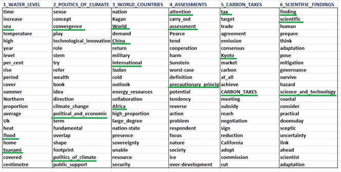
Ordered
according to their Chi-square values, the most relevant
words of twelve themes are listed below (N.B.: Each theme is labelled
by using some of its typical key-words. More specifically, even if T-LAB
automatically suggests 'its' labels, in this case each one of them has been
assigned manually by using a specific feature of the software).
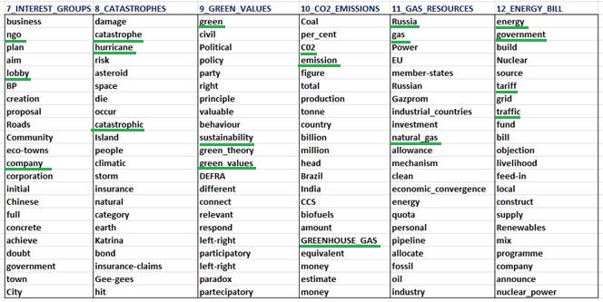
Fig.
8
Click
here to see the two most typical text segments of each thematic cluster
(measure = chi-square test),
(N.B.: the listed text segments can also be used for a sort of text summarization).
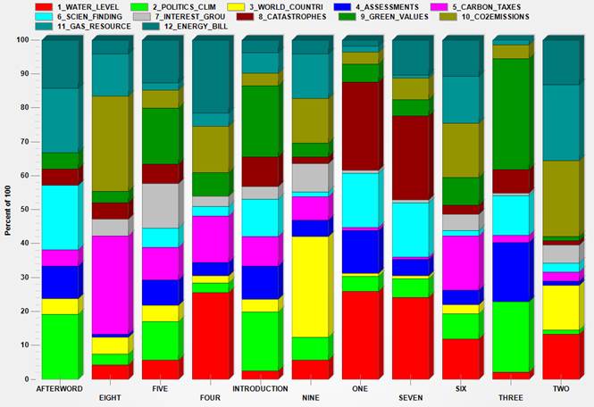
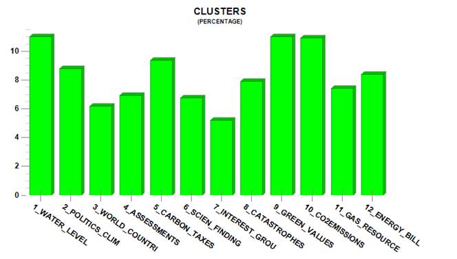
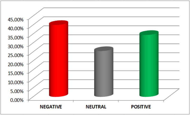
The relative weights
of the twelve thematic clusters, which correspond to the percentage
of text segments falling into each of them, are summarized by the following
chart.
Fig.
9
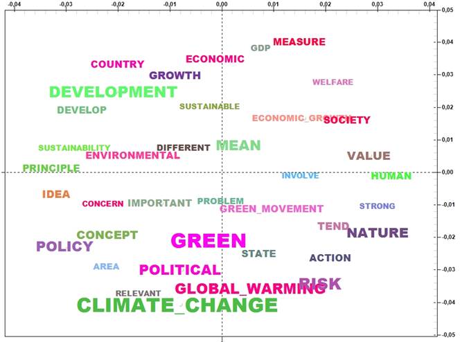
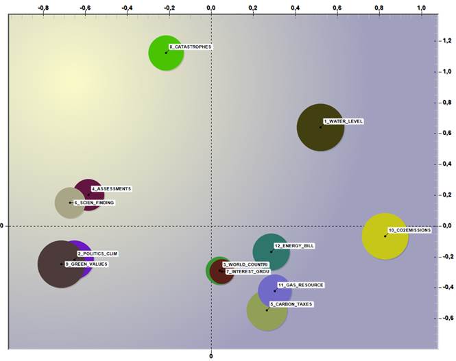
The way the twelve
themes are framed into the semantic space of the first
two factors is the following:
Fig.
10
The
twelve themes
cross the eleven sections of the book is
the following way:
Fig.
11
So, for
example, the main themes of chapter eight (the
title of which is 'International Negotiations, the EU and Carbon Market’)
result to be ‘CO2_EMISSIONS’ and ‘CARBON_TAXES’.
SECTION
3: DEALING WITH THE SEQUENCES OF THEMES
Starting
from the version 9.1, T-LAB
includes a new tool which – when the corpus consists of subsets
ordered in a sequential fashion (e.g. chapters of a book, parts of an
interview, turns in a conversation or a debate, etc.) – allow us to map
the sequences of themes in quite an interesting
way.
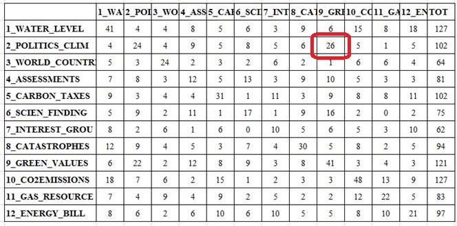
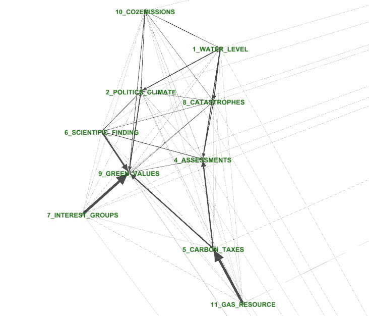
To start
with, let’s examine the following matrices
(see Fig. 12 and Fig. 13 below) which cross the twelve themes with each other.
More
specifically, the numbers in Fig. 12 indicate how many times each theme in a
row precedes each theme in a column. For example, POLITICS_CLIMATE
results to be a predecessor of GREEN_VALUES
twenty-six times. That means that – according to the T-LAB analysis –
26 text segments classified as belonging to the GREEN_VALUES
theme are successors of text segments classified
as belonging to the POLITICS_CLIMATE theme.
Fig.
12
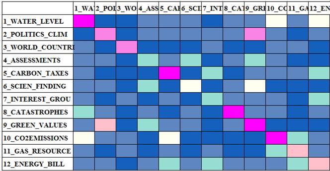
As one
could intuit, the most frequent cases are those where both the predecessor and
the successor refer to the same theme (see the diagonal
of both matrices). In fact, when ‘engaged’
in a specific theme, arguably the author has spent more than a couple sentences
(and one after the other) on such a theme.
Fig.
13
In other
words, such a tool allows the user to perform a specific kind of ‘discourse
analysis’ which takes into account the theme sequences.
Actually
these kinds of sequences can also be tracked by means of animated
charts either referring to the entire corpus or to a subset of it.
For example, by clicking the below pictures it
is possible to track how the thematic discourse evolves within chapter three
of the Giddens book.
More specifically:
- the
3d matrix, which crosses the twelve themes with
each other, shows how each transition (i.e. predecessor --> successor) increases
over time;
- the
2d chart, the abscissa and the ordinate of which
correspond to the factorial axes selected by the user, shows how the dimension
(i.e. percentage) of each theme varies over time. Meanwhile moving arrows indicate
how themes follow each other.
Fig.
14
Fig.
15
Last
but not least, as T-LAB allows the user to save
some files (e.g.: .dl, .gml, .net, .vna formats) which can be easily imported
by software for network analysis like Gephi (http://gephi.org/)
and
many others, a graph like the following can be quickly obtained.
This website uses cookies so that we can provide you with the best user experience possible. Cookie information is stored in your browser and performs functions such as recognising you when you return to our website and helping our team to understand which sections of the website you find most interesting and useful.
Strictly Necessary Cookies
Strictly Necessary Cookie should be enabled at all times so that we can save your preferences for cookie settings.
If you disable this cookie, we will not be able to save your preferences. This means that every time you visit this website you will need to enable or disable cookies again.
3rd Party Cookies
This website uses Google Analytics to collect anonymous information such as the number of visitors to the site, and the most popular pages.
Keeping this cookie enabled helps us to improve our website.
Please enable Strictly Necessary Cookies first so that we can save your preferences!